1  Base R

1.1 Short Glossary

Let’s start the tutorial with a (very) short glossary:

• Console: The thing with the > sign at the beginning.
• Script file: An ordinary text file with suffix .R. For instance, yourfilename.R.
• Working directory: The file directory you are working in. If no directory is explicitly specified when loading data, then R assumes that the data is located in the working directory. Useful commands: with getwd(), you get the location of your current working directory, and setwd() allows you to set a new location for it.
• Workspace: This is a hidden file (stored in the working directory as .RData) where all objects you use (e.g., data, matrices, vectors, variables, functions, etc.) are stored. When you close RStudio, you will be asked if you want to save or delete the session’s workspace. If you save it, it will be loaded automatically with the next R session, provided you start R in the corresponding working directory. Useful commands: ls() shows all elements in our current workspace, and rm(list=ls()) deletes all elements in our current workspace.

1.2 First Steps

A good idea is to use a script file like myscipt.R to store your R commands. You can send single lines or marked areas of your R code to the console by pressing the CTRL+RETURN (STRG+ENTER) keys.

To start with baby steps, we do some simple calculations:

2+2 # addition

[1] 4

2*2 # multiplication

[1] 4

2/2

[1] 1

2-2

[1] 0

2^3 # exponentiate

[1] 8

Note: Anything written after the # sign will be ignored by R, which is very useful for commenting on your code.

The assignment operator <- will be your most often-used tool. Here is an example of creating a scalar variable:

x <- 4 
x

[1] 4

4 -> x # possible but unusual
x

[1] 4

x = 4
x

[1] 4

Note: The R community loves the <- assignment operator. Alternatively, you can use the = operator.

1.3 Vectors and functions

And now a more interesting object - a vector:

y = c(2,7,4,1)
y

[1] 2 7 4 1

The command ls() shows the total content of your current workspace, and the command rm(list=ls()) deletes all elements of your current workspace:

ls()

[1] "has_annotations" "x"               "y"              

rm(list=ls())
ls()

character(0)

Note: RStudio’s Environment pane also lists all the elements in your current workspace. That is, the command ls() becomes a bit obsolete when working with RStudio.

Let’s try how we can compute with vectors and scalars in R.

x = 4
y = c(2,7,4,1)

x*y # each element in the vector y is multiplied by the scalar x

[1]  8 28 16  4

y*y # a term-by-term product of the elements in y

[1]  4 49 16  1

The term-by-term execution, as in the above example, y*y, is a main strength of R. We can conduct many operations vector-wisely:

y^2

[1]  4 49 16  1

log(y)

[1] 0.6931472 1.9459101 1.3862944 0.0000000

exp(y)

[1]    7.389056 1096.633158   54.598150    2.718282

y-mean(y)

[1] -1.5  3.5  0.5 -2.5

(y-mean(y))/sd(y) # standardization 

[1] -0.5669467  1.3228757  0.1889822 -0.9449112

Element-wise operations are a central characteristic of matrix-based languages like R (or Matlab). Other programming languages often have to use loops instead:

N = length(y)
1:N

y.sq = rep(0,N)
y.sq

for(i in 1:N){
  y.sq[i] = y[i]^2
  if(i == N){
    print(y.sq)
  }
}

The for()-loop is the most common loop, but there is also a while()-loop and a repeat()-loop. However, loops in R can be relatively slow. Therefore, try to avoid them!

Useful commands to produce sequences of numbers:

1:10
-10:10
?seq # Help for the seq()-function
seq(from=1, to=100, by=7) # sequence generation
rep(0,10) # replicate elements

The []-operator selects elements of vectors:

y[c(2,4)]

[1] 7 1

Element selections can be made on a more logical basis, too. For example, if you want only the elements of the vector y that are strictly greater than 2:

y[y>2]

[1] 7 4

# Note that this gives you a boolean vector:
y>2

[1] FALSE  TRUE  TRUE FALSE

Note: Logical operations return so-called boolean objects, i.e., a TRUE or a FALSE. For instance, if we ask R whether 1>2, we get the answer FALSE.

1.4 Further Data Objects

Besides the classical data objects like scalars and vectors, there are many other objects in R:

1.4.1 The matrix

A matrix is a rectangular array of numbers.

mymatrix = matrix(data=1:16, nrow=4, ncol=4)
mymatrix

     [,1] [,2] [,3] [,4]
[1,]    1    5    9   13
[2,]    2    6   10   14
[3,]    3    7   11   15
[4,]    4    8   12   16

Matrices are extremely useful for theoretically analyzing statistical methods and implementing them practically.

Matrix Algebra in R

To refresh your matrix algebra skills with implementations in R, check out my Crash Course on Matrix Algebra in R.

1.4.2 The list

In lists, you can organize different kinds of data. E.g., consider the following example:

mylist = list(
  "Some_Numbers" = c(66, 76, 55, 12, 4, 66, 8, 99), 
  "Animals"      = c("Rabbit", "Cat", "Elefant"),
  "My_Series"    = c(30:1)
) 

A very useful function to find specific values and entries within lists is the str()-function:

str(mylist)

List of 3
 $ Some_Numbers: num [1:8] 66 76 55 12 4 66 8 99
 $ Animals     : chr [1:3] "Rabbit" "Cat" "Elefant"
 $ My_Series   : int [1:30] 30 29 28 27 26 25 24 23 22 21 ...

1.4.3 The data frame

A data.frame is a list object with more formal restrictions (e.g., an equal number of rows for all columns). As indicated by its name, a data.frame object is designed to store data:

mydataframe = data.frame(
  "Credit_Default"   = c( 0, 0, 1, 0, 1, 1), 
  "Age"              = c(35,41,55,36,44,26), 
  "Loan_in_1000_EUR" = c(55,65,23,12,98,76)
) 

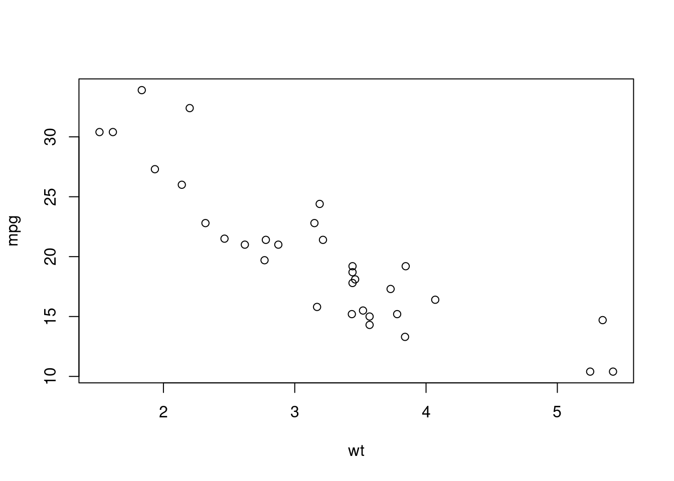
The data() command lists all sample data sets available in R. Let us have a look at the dataset mtcars. It is a dara.frame object and contains data on several aspects of 32 automobiles from 1974.

mtcars

                     mpg cyl  disp  hp drat    wt  qsec vs am gear carb
Mazda RX4           21.0   6 160.0 110 3.90 2.620 16.46  0  1    4    4
Mazda RX4 Wag       21.0   6 160.0 110 3.90 2.875 17.02  0  1    4    4
Datsun 710          22.8   4 108.0  93 3.85 2.320 18.61  1  1    4    1
Hornet 4 Drive      21.4   6 258.0 110 3.08 3.215 19.44  1  0    3    1
Hornet Sportabout   18.7   8 360.0 175 3.15 3.440 17.02  0  0    3    2
Valiant             18.1   6 225.0 105 2.76 3.460 20.22  1  0    3    1
Duster 360          14.3   8 360.0 245 3.21 3.570 15.84  0  0    3    4
Merc 240D           24.4   4 146.7  62 3.69 3.190 20.00  1  0    4    2
Merc 230            22.8   4 140.8  95 3.92 3.150 22.90  1  0    4    2
Merc 280            19.2   6 167.6 123 3.92 3.440 18.30  1  0    4    4
Merc 280C           17.8   6 167.6 123 3.92 3.440 18.90  1  0    4    4
Merc 450SE          16.4   8 275.8 180 3.07 4.070 17.40  0  0    3    3
Merc 450SL          17.3   8 275.8 180 3.07 3.730 17.60  0  0    3    3
Merc 450SLC         15.2   8 275.8 180 3.07 3.780 18.00  0  0    3    3
Cadillac Fleetwood  10.4   8 472.0 205 2.93 5.250 17.98  0  0    3    4
Lincoln Continental 10.4   8 460.0 215 3.00 5.424 17.82  0  0    3    4
Chrysler Imperial   14.7   8 440.0 230 3.23 5.345 17.42  0  0    3    4
Fiat 128            32.4   4  78.7  66 4.08 2.200 19.47  1  1    4    1
Honda Civic         30.4   4  75.7  52 4.93 1.615 18.52  1  1    4    2
Toyota Corolla      33.9   4  71.1  65 4.22 1.835 19.90  1  1    4    1
Toyota Corona       21.5   4 120.1  97 3.70 2.465 20.01  1  0    3    1
Dodge Challenger    15.5   8 318.0 150 2.76 3.520 16.87  0  0    3    2
AMC Javelin         15.2   8 304.0 150 3.15 3.435 17.30  0  0    3    2
Camaro Z28          13.3   8 350.0 245 3.73 3.840 15.41  0  0    3    4
Pontiac Firebird    19.2   8 400.0 175 3.08 3.845 17.05  0  0    3    2
Fiat X1-9           27.3   4  79.0  66 4.08 1.935 18.90  1  1    4    1
Porsche 914-2       26.0   4 120.3  91 4.43 2.140 16.70  0  1    5    2
Lotus Europa        30.4   4  95.1 113 3.77 1.513 16.90  1  1    5    2
Ford Pantera L      15.8   8 351.0 264 4.22 3.170 14.50  0  1    5    4
Ferrari Dino        19.7   6 145.0 175 3.62 2.770 15.50  0  1    5    6
Maserati Bora       15.0   8 301.0 335 3.54 3.570 14.60  0  1    5    8
Volvo 142E          21.4   4 121.0 109 4.11 2.780 18.60  1  1    4    2

With the function subset we can select variables and subsets of a dataframe. Let’s create a scatterplot of the variables mpg (miles per gallon) and wt weight (in 1000 lbs).

plot(subset(mtcars, select = c(wt, mpg)))

A data.frame is also useful in a time series context. Since time series data typically include a calendar date for each observation, the observation and date can be stored together as a data.frame. R provides the class Date for calendar dates, which can be generated with the function as.Date().

d = as.Date("2021-04-01") # a data object to store dates
class(d) # to get the object class

[1] "Date"

myseries = c(16,17,18,16,15,19)
mydates = seq.Date(as.Date("2021-04-01"), by=1, length.out = 6)
mytimeseries = data.frame(mydates, myseries)
mytimeseries

     mydates myseries
1 2021-04-01       16
2 2021-04-02       17
3 2021-04-03       18
4 2021-04-04       16
5 2021-04-05       15
6 2021-04-06       19

1.4.4 The ts object

A ts (time series) object is tailored explicitly to time series with a yearly time basis and an equidistant observation horizon, such as annual, quarterly, and monthly data. It assigns a specific year/quarter/month to each vector entry.

myts = ts(c(66, 76, 55, 12, 4, 66, 8, 99), start = 2020, frequency = 4)
myts

     Qtr1 Qtr2 Qtr3 Qtr4
2020   66   76   55   12
2021    4   66    8   99

anothertimeseries = ts(1:50, start = 2015, frequency = 12)
anothertimeseries

     Jan Feb Mar Apr May Jun Jul Aug Sep Oct Nov Dec
2015   1   2   3   4   5   6   7   8   9  10  11  12
2016  13  14  15  16  17  18  19  20  21  22  23  24
2017  25  26  27  28  29  30  31  32  33  34  35  36
2018  37  38  39  40  41  42  43  44  45  46  47  48
2019  49  50                                        

# The window() command selects the time series observations for a given subperiod
window(anothertimeseries, start=2015.5, end=2017.5)

     Jan Feb Mar Apr May Jun Jul Aug Sep Oct Nov Dec
2015                           7   8   9  10  11  12
2016  13  14  15  16  17  18  19  20  21  22  23  24
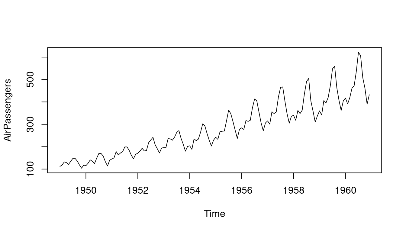
2017  25  26  27  28  29  30  31                    

The data() command lists all sample data sets available in R. Let us have a look at the dataset AirPassengers. It is a ts object and contains data on monthly totals of international airline passengers from 1949 to 1960.

data() # lists all datasets currently loaded in the R environment
?AirPassengers # get more information about the dataset
AirPassengers

     Jan Feb Mar Apr May Jun Jul Aug Sep Oct Nov Dec
1949 112 118 132 129 121 135 148 148 136 119 104 118
1950 115 126 141 135 125 149 170 170 158 133 114 140
1951 145 150 178 163 172 178 199 199 184 162 146 166
1952 171 180 193 181 183 218 230 242 209 191 172 194
1953 196 196 236 235 229 243 264 272 237 211 180 201
1954 204 188 235 227 234 264 302 293 259 229 203 229
1955 242 233 267 269 270 315 364 347 312 274 237 278
1956 284 277 317 313 318 374 413 405 355 306 271 306
1957 315 301 356 348 355 422 465 467 404 347 305 336
1958 340 318 362 348 363 435 491 505 404 359 310 337
1959 360 342 406 396 420 472 548 559 463 407 362 405
1960 417 391 419 461 472 535 622 606 508 461 390 432

class(AirPassengers)  # AirPassengers is a ts object

[1] "ts"

plot(AirPassengers)